Contents
What the diagram shows
Curvature is the rotation per unit length of a member’s axis: κ = 1/r, the inverse of the radius of curvature. Because plane sections remain plane, it is also the strain gradient over the depth. With a compressive strain εc at the top and a tensile strain εs in the reinforcement at depth d, κ = (εc + εs) / d.
For a linear-elastic material the relation is a straight line, M = EI · κ. Reinforced concrete is not linear: it cracks, the steel yields and the concrete crushes. The M-κ diagram records that behaviour in one curve, in three stages.
- Uncracked (state I). Concrete and steel act together and the stiffness is EcmII. This stage ends at the cracking moment Mcr, when the tensile stress reaches fctm.
- Cracked (state II). At a crack the concrete in tension no longer counts, and the stiffness drops, often to a quarter or a third of the uncracked value. Between the cracks the concrete still carries some tension (tension stiffening), so the real curve lies between the uncracked and the fully cracked line.
- Yielding and failure. Once the reinforcement yields, the moment hardly rises while the curvature keeps growing, until the concrete reaches its ultimate strain εcu at the compression face. That point gives the moment resistance and the curvature capacity, a measure of ductility.
What a beam or frame analysis needs is the secant stiffness EIsec = M / κ at the moment that actually occurs. It depends on that moment, which is why cracked concrete is physically non-linear.
Why the axial force N matters
An axial force changes every point of the curve. Compression delays cracking, because the bending first has to overcome it. It raises the moment resistance up to the balanced point, where the steel yields just as the concrete crushes; beyond that point more compression lowers the resistance again. And it reduces the curvature at failure: the section becomes stronger but less ductile.
So one cross-section has a family of curves, one for each value of N: an M-N-κ diagram. FIG. 1 shows three of them for the section of the worked example below.
How the diagram is calculated
The calculation uses the assumptions of EN 1992-1-1 §6.1(2): plane sections remain plane, bonded reinforcement has the same strain as the concrete around it, and each material follows its own stress-strain curve. One point of the diagram takes four steps.
- Choose a curvature κ.
- Find the strain at the top fibre for which the internal forces add up to the applied axial force N. This needs iteration, because the stress-strain curves are non-linear.
- Integrate the stresses of that strain distribution over the section to get the moment M.
- Repeat for increasing κ until the concrete or the steel reaches its strain limit.
Software does this with a fibre model: the concrete is divided into thin layers and each reinforcing bar is a point. Any shape can be handled this way, from T-beams to hollow sections and walls with reinforcement in several layers.
Which stress-strain curves to use
That depends on what the diagram is for. Using the wrong set is the most common mistake with M-κ diagrams.
| Purpose | Concrete | Reinforcement | Clause |
|---|---|---|---|
| Deflection, short-term (SLS) | mean values: Ecm; cracking at fctm | elastic, Es = 200 000 N/mm² | §7.4.3 |
| Deflection, long-term (SLS) | effective modulus Ec,eff = Ecm / (1 + φ(∞,t0)) | as above | §7.4.3 (7.20) |
| Resistance of the section (ULS) | design curve (parabola-rectangle or bilinear), fcd = αccfck / γc; tension ignored | design curve, fyd = fyk / γs | §3.1.7, §3.2.7, §6.1 |
| Non-linear analysis of slender columns | curve (3.14) with fcd and Ecd = Ecm / γcE; creep included | design values | §3.1.5, §5.8.6 |
γcE = 1.2 is the recommended value in §5.8.6(3); the national annex may set another. In the Dutch annex αcc = 1.0.
For a deflection the diagram describes the expected behaviour, so it uses mean material values. For the resistance, the partial factors are already in the curves, and the top of the diagram is the design moment resistance MRd.
Worked example: a rectangular beam
A beam of 300 × 500 mm in C30/37, with 3Ø20 in B500B at the bottom: As = 942 mm², d = 450 mm, no axial force. From Table 3.1: fctm = 2.9 N/mm² and Ecm = 33 000 N/mm². To keep the hand calculation short, the uncracked stiffness uses the gross concrete section; including the reinforcement would raise it by a few per cent.
β = 1.0 applies to a single short-term load. For sustained or often repeated loading §7.4.3(3) takes β = 0.5, which gives ζ = 0.82 and EIsec = 30.3 MNm² at the same moment. FIG. 2 shows the short-term curve from zero to 160 kNm.
This is the top of the ULS curve for N = 0 in FIG. 1, where the fibre model finds the same 170.0 kNm.
What the diagram is used for
Deflection of concrete beams
Along a beam the moment varies, and so does the stiffness: near the supports of a simply supported beam the concrete is uncracked, at midspan it is cracked. §7.4.3(7) names the most rigorous method: compute the curvature at frequent sections along the member and integrate it numerically to a deflection. An M-κ diagram gives each section the curvature that belongs to its moment.
In a statically indeterminate beam there is a second effect. The stiffness also changes the distribution of the moments, because cracked regions attract less moment. A physically non-linear analysis iterates until moments and stiffnesses agree.
Slender columns and second-order effects
In a slender column the additional moment from the deflection depends on the stiffness, and the stiffness depends on the moment and the axial force. The general method of §5.8.6 solves this with a non-linear analysis based on this behaviour, including creep. The nominal stiffness method (§5.8.7) and the nominal curvature method (§5.8.8) are simplifications of the same idea.
Checking a stiffness assumption
Frame models often use a reduced EI for cracked concrete members. The diagram shows what that reduction really is for a given section, moment and axial force, instead of a rule of thumb.
M-N-κ in XConstruct and XBeam2D
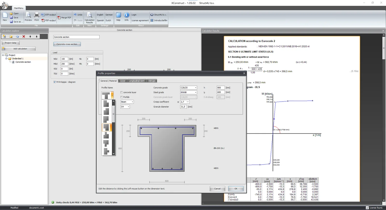
XConstruct has a concrete module with an integrated M-N-κ diagram, for all types of concrete cross-section. It also gives the stiffness EI at a moment MEd you enter, and since version 2025-01-01 (September 2024) it shows the diagram for both short-term and long-term loading.
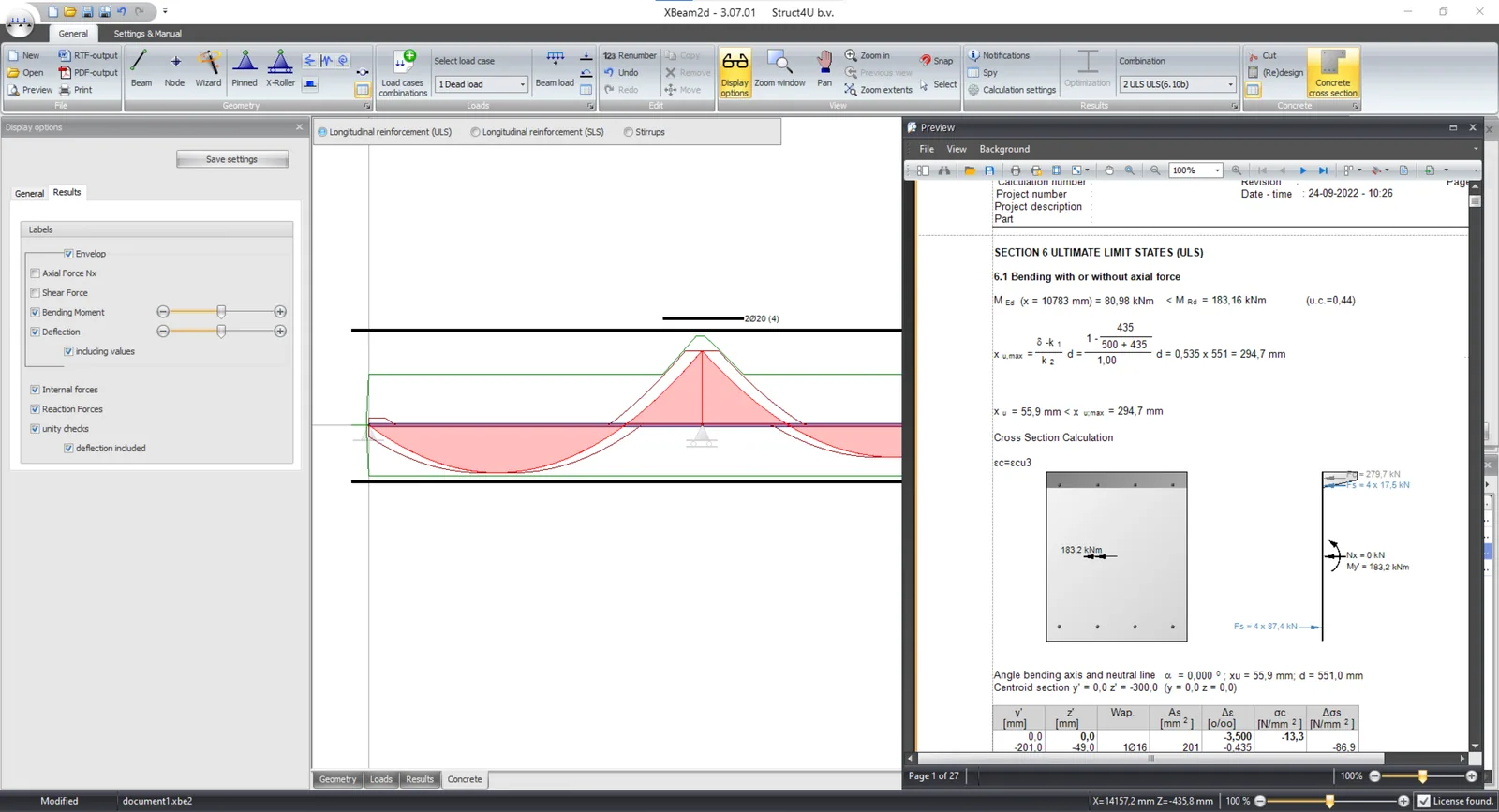
The diagram is also integrated in XBeam2D. As a result, the deflection calculation in XBeam2D is physically non-linear: for each point of the beam the program takes the stiffness that belongs to the bending moment there, and uses it for both the distribution of forces and the deflection. All formulas that go into the result are shown in the output, so the calculation stays fully transparent.
Common mistakes
- The design curve for a deflection. The partial factors make the section look softer and weaker than it is, and ignoring the tensile strength removes the uncracked stage altogether.
- No creep. Under sustained load the curvature grows with time. Use Ec,eff from (7.20) for the long-term curve.
- The fully cracked stiffness everywhere. It ignores tension stiffening and the uncracked zones, so it overestimates the deflection, just as the gross stiffness underestimates it.
- No axial force. A column or a prestressed member has a very different curve from the same section in pure bending.
- EN 1992-1-1:2004, Eurocode 2: Design of concrete structures, Part 1-1 (in the Netherlands NEN-EN 1992-1-1+C2:2011 with its national annex): §3.1.5, §3.1.7, §3.2.7, §5.8.6–5.8.8, §6.1, §7.4.3.
- Struct4U, “M-N-kappa diagram”, struct4u.com, 10 June 2022: the post this article replaces.
- Struct4U, release notes XConstruct (opens in a new tab): version 1.02.02 (EI at a given moment) and version 2025-01-01 of 21 September 2024 (short-term and long-term diagrams).
Originally published on struct4u.com on .